I built a world model from scratch.

About a month ago I got curious about world models. Not the “AGI is coming” kind, the 2018 Ha and Schmidhuber kind: a neural net that learns to simulate its own environment, then trains a tiny agent inside that simulation. They solved CarRacing with a controller that had fewer than a thousand parameters. I wanted to see if I could reproduce it in 2026, on a laptop, in a weekend.

This is how that went.

What a world model actually is

Most RL agents look at a screen, run it through a big neural network, and spit out an action. The network has to learn perception, memory, and control all at once, from a very sparse reward signal. That is hard. It needs a lot of data and a lot of compute.

A world model splits that job three ways.

First, a vision module that compresses each frame into a small latent vector. In this project, 64 by 64 RGB goes down to 32 floats. The vision module trains on pixel reconstruction, not reward, so it has dense feedback for every frame.

Second, a dynamics model that learns to predict the next latent given the current latent and the agent’s action. This is the dream. Once trained, you can start with one real frame, roll forward 80 steps using only the dynamics model, decode each predicted latent back to pixels, and the video looks convincingly like real gameplay.

Third, a tiny controller that takes the latent and the dynamics model’s hidden state and outputs an action. Because perception and dynamics are already handled by the other two networks, the controller doesn’t need to be big. Mine has 867 parameters total.

The split means each network learns from a dense, specific signal. The hard sparse reward only has to teach a thousand numbers.

Setup, and one afternoon I almost wasted

I run an M3 Pro Mac. I had Python 3.12 installed through miniforge from some older project. I set up the venv, installed PyTorch, and started training.

The first VAE run was taking forever. I opened Activity Monitor and saw Python pegging a single CPU core while the GPU sat at zero. torch.backends.mps.is_available() returned True. But training was clearly not on the GPU.

The problem turned out to be Rosetta. My miniforge Python was an x86_64 binary running in emulation. platform.machine() returned x86_64 even though the hardware was arm64. PyTorch’s MPS backend only works on a native arm64 Python. So MPS was sort of “available” but not doing anything useful.

The fix was rebuilding the venv against /opt/homebrew/bin/python3.12, which is natively arm64. After that, training dropped from about four hours estimated to about 35 minutes total for the full pipeline.

Collecting data

CarRacing-v3 is the Gymnasium version of the old OpenAI Gym environment. Top-down view, a red car, a procedurally generated track. The action space is continuous: steering, gas, brake.

I ran 200 random episodes, saving every frame, action, and reward. Small trick I learned from the original paper. Pure random actions cause the car to spin in place, which gives you very little useful data. Repeating the same action for four steps before sampling a new one gives the agent enough momentum to actually drive around and explore the track.

Total: 95,169 frames, 115 MB raw. Took about five minutes to collect. This is the only time the agent interacts with the real environment for training the perception and dynamics networks. Everything downstream runs on the latent representation.

The VAE

The VAE has four strided convolutions in the encoder going from 64 by 64 down to 2 by 2, then two linear heads that produce a mean vector and a log-variance vector, each 32-dimensional. The decoder mirrors the encoder and ends in a sigmoid.

The loss has two parts. First, pixel-wise MSE between the input and the reconstruction. Second, the KL divergence between the encoder’s output distribution and a standard normal prior.

The KL term is what makes the latent space useful. Without it you just have a deterministic autoencoder and the latent vectors end up weird, clumpy, and not something a dynamics model can easily learn to predict. The KL pulls the encoder toward a smooth, well-shaped latent where nearby vectors decode to visually similar frames.

Trained ten epochs on the 95K frames at batch size 128. Loss went from 163 to 31 and was still trending down. I stopped because the reconstructions already looked clean enough to keep going.

The MDN-RNN

This is the part I think is most elegant in the whole system. The dynamics model doesn’t predict a single next latent. It predicts a mixture of five Gaussian distributions over the next latent, each with its own mean, variance, and mixing weight.

The reason you need the mixture: real environments branch. Given the current state and action, the next state might go one of several distinct ways. A single Gaussian would be forced to average over those futures, and the average of two distinct outcomes often matches neither of them. The mixture lets the model represent branching explicitly. At sampling time, you pick a component by its weight, then sample from its Gaussian.

The model is an LSTM with 256 hidden units. At each step it takes the current latent (32) concatenated with the current action (3), total 35 dimensions in. It outputs 325 numbers: five weights, five 32-dim means, five 32-dim log standard deviations, plus a predicted reward.

Loss is the negative log-likelihood of the true next latent under the predicted mixture. Trained 20 epochs on pre-encoded latent sequences, which dropped the storage footprint from 115 MB of frames to 22 MB of latents, and let training iterate about 20x faster.

One small thing I had to debug. My initial dataset was too small per epoch, about three batches. Training looked like it was overfitting instantly. The fix was to sample ten random sub-sequences per episode instead of one, which expanded the effective epoch size to about 30 batches and gave the loss curve a clean declining shape.

Is the dream actually working

This was the moment I knew the project was working.

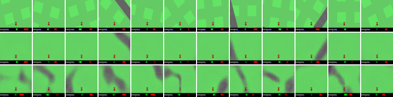
I took a real episode. Encoded frame 0 through the VAE to get z_0. Fed (z_0, a_0) into the MDN-RNN, sampled z_1. Then, instead of using the real frame 1, I fed my sampled z_1 plus a_1 into the MDN-RNN to get z_2. And so on for 80 steps. Then I decoded every z back through the VAE.

The result is an 80-step dream rollout: what the world model thinks the next 80 frames look like, given only the first frame and the actions the real agent took. If the dynamics model were bad, compounding errors would diverge fast. Within 10 or 20 steps the dream would look nothing like reality.

Mine tracks the real episode for the full 80 steps. Same turns, same road layout, same car orientation.

The controller

867 parameters. One linear layer from [z; h] (288 dimensions) to a 3-dim action, with tanh on the steering output and sigmoid on gas and brake to match the environment’s expected action range. That’s it. No hidden layer, no fancy head.

I trained it with CMA-ES, covariance matrix adaptation evolution strategy. The library cma on PyPI is the standard implementation. The reason to use evolution instead of gradient-based RL: the environment is not differentiable, the reward is noisy, and the controller is small enough that CMA-ES handles it easily. PPO would work too, probably give less variance in the final result, but at the cost of ripping through a lot more code.

Population 16, two rollouts per individual, 30 generations. Each generation samples 16 candidate parameter vectors, runs each in the real environment twice, averages the returns, and updates a multivariate Gaussian over parameter space so the next generation concentrates around good candidates.

Total training time: about 20 minutes. The return curve looked like this:

• Generation 1: mean 1.4, best 8.4
• Generation 15: mean 43, best 264
• Generation 30: mean 121, best 343

The final saved controller, evaluated on fresh random seeds: best single-episode return of 881. CarRacing is considered solved at an average of 900 over 100 episodes. I’m not there yet on average, but the single-episode peak shows the system can drive a full track.

What I’d change next time

Four things, in rough order of how much I think each would help.

More rollouts. 200 is on the low end. 2000 would give the VAE and MDN-RNN a richer training distribution and probably tighten up the dream.

Iterative data. Collect initial rollouts with a random policy, train the world model, run the trained controller, collect new rollouts, retrain. The trained controller visits different regions of state space than a random one, and the world model gets sharper where it matters.

Train the controller in the dream. This is the DreamerV3 move. Once you have a good world model, you can train a policy with PPO entirely on simulated rollouts, which is dramatically more sample-efficient than running every evaluation in the real environment.

A discrete latent. DreamerV3 replaced the continuous Gaussian latent with a discrete categorical one and argued it generalizes better across tasks. Worth trying.

What this taught me

The big takeaway is the architectural one: decomposing a hard learning problem by signal density. Sparse reward teaches 867 parameters. Dense pixel loss teaches 4.3 million. That ratio is what makes the whole thing tractable on a laptop.

The repo is on GitHub at abhi183/world-model. About 1,500 lines of Python spread across the model modules and training scripts. If you want to reproduce, the README has a one-command path from empty venv to a trained agent.